
Using transfer learning with VGG19 to Classify Grapevines Leaves — Part 1

Hi guys, today I’ll show you how to use VGG19 to classify grape leaves using transfer learning. In this part we’ll focus on how to build the model, and in part 2 I’ll show you how to deploy this model with streamlit.
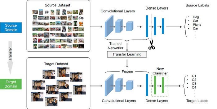
What is transfer learning?
The goal in transfering learning is that you don’t have to train a new model from scratch, it is about leveraging feature representations from a pre-trained model.
The pre-trained models are usually trained on massive datasets that are a standard benchmark in the computer vision frontier. The weights obtained from the models can be reused in other computer vision tasks.
These models can be used directly in making predictions on new tasks or integrated into the process of training a new model. Including the pre-trained models into a new model that leads to lower training time and lower generalization error.
Transfer learning is particularly very useful when you have a small training dataset, ans this is our case (I’ll show you later). In this case, you can, for example, use the weights from the pre-trained models (VGG19) to initialize the weights of the new model.
VGG19:
VGG-19 is a convolutional neural network that is 19 layers deep. We can load a pretrained version of the network trained in more than a million images from the ImageNet database. The pretrained network can classify images into 1000 object categories, such as keyboard, mouse, pencil, and many animals. As a result, the network has learned rich feature representations for a wide range of images. The network has an image input size of 224-by-224.
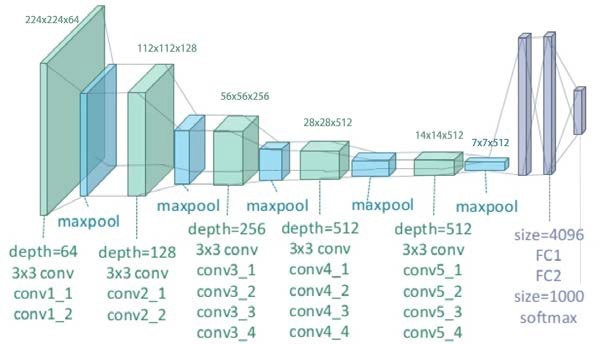
Architecture
A fixed size of (224 * 224) RGB image was given as an input to this network which means that the matrix was of a shape of 224x224x3.
The only preprocessing that was done is that they subtracted the average RGB value from each pixel, computed over the whole training set.
Used kernels of 3x3 size with a stride size of 1 pixel, this enabled them to cover the whole notion of the image.
Spatial padding was used to preserve the spatial resolution of the image.
Max pooling was performed over a 2x2 pixel window with stride 2.
This was followed by Rectified linear unit (ReLu) to introduce non-linearity to make the model classify it better and to improve computational time as the previous models used tanh or sigmoid functions which proved to be much better than those.
Implemented three fully connected layers from which the first two were of size 4096 and after that a layer with 1000 channels for 1000 ILSVRC-ways to classify the image, and the final layer is a softmax function.
Repository:
Our dataset is about Grapevine Leaves and our goal is to classify this leaves by deep leaning using VGG19.
The main product of grapevines are grapes that are consumed fresh or processed. In addition, grapevine leaves are harvested once a year as a by-product. The species of grapevine leaves are important in terms of price and taste. We can use deep learning based classification to conduct it using images of grapevine leaves. For this purpose, images of 500 (it’s a small dataset) vine leaves belonging to 5 species which were taken with a special self-illuminating system. The 5 species are : AK, Ala Idris, Buzgulu, Dimnit and Nazil

Code:
So, let’s go to our code. The first thing to do is to download our dataset. Ah! Everything that we’ll do is made in google colab environment. If we go to the kaggle.com, you can download your json credentials, so do this and upload this file in your colab, because we’ll use this to download the dataset. After, execute the code below.
import os# Lendo as crendenciais para download do dataset
os.environ['KAGGLE_CONFIG_DIR'] = "/content"
!chmod 600 /content/kaggle.json# Download do dataset
!kaggle datasets download -d muratkokludataset/grapevine-leaves-image-dataset# #Descompressao do dataset
!unzip /content/grapevine-leaves-image-dataset.zip -d /content/kaggle/
After, we’ll import the libraries.
import os
import numpy as np
import cv2
import random
import pandas as pd
import seaborn as sns
from tqdm import tqdm
from matplotlib import pyplot as plt
from sklearn.preprocessing import LabelEncoder, LabelBinarizer
from sklearn.model_selection import train_test_split
from sklearn.metrics import classification_report,confusion_matriximport tensorflow
import keras
from keras.callbacks import ReduceLROnPlateau, ModelCheckpoint, EarlyStopping, TensorBoard
from keras.applications.vgg19 import VGG19
from keras.models import Sequential, Model
from keras.layers import Dense, Conv2D , MaxPool2D , Flatten , Dropout , MaxPooling2Dtensorflow.__version__
Ok! Now we need to read our pictures and organize them. I’ll put the path to our images and respective labels on pandas Dataset.
labels = ['Ak', 'Ala_Idris', 'Buzgulu', 'Dimnit', 'Nazli']
base_dir = '/content/kaggle/Grapevine_Leaves_Image_Dataset/'print(os.listdir(base_dir))
path = []
label = []for grape_class in os.listdir(base_dir):
    label_path = os.path.join(base_dir, grape_class)
    if grape_class in labels:
        for img in os.listdir(label_path):
            path.append(os.path.join(label_path, img))
            label.append(grape_class)path = pd.Series(path)
labels = pd.Series(label)
img_data = pd.DataFrame({'Path':path.values, 'Label':labels.values})print(img_data.head())
print(img_data.shape)
Next, we’ll plot some images and labels. That’s all.
plt.figure(figsize=(10,10))
rand_indicies = np.random.randint(len(img_data), size=25)
for i in range(25):
    plt.subplot(5,5,i+1)
    plt.xticks([])
    plt.yticks([])
    plt.grid(False)
    index = rand_indicies[i]
    plt.imshow(cv2.imread(img_data.iloc[index]['Path']), cmap=plt.cm.binary)
    plt.xlabel(img_data.iloc[index]['Label'])
plt.show()
So, now it’s time to do the magic. The first thing we need to do is to label the encoder, because our model needs to know the label by numeric form.
labelencoder = LabelEncoder()img_data['Categorical'] = labelencoder.fit_transform(img_data['Label'])The next step is the traditionally splitting our dataset, but we don’t use sklearn here yet in training, testing and validing. The validing dataset are images that our model has never seen before.
img_data = img_data.sample(frac=1).reset_index(drop=True)train_df = img_data[:450]
valid_df = img_data[450:]img_size = 224data = []for img, label in zip(train_df['Path'], train_df['Categorical']):
  # print(img, label)
  img_arr = cv2.imread(img, cv2.IMREAD_COLOR)
  resized_arr = cv2.resize(img_arr, (img_size, img_size))
  data.append([resized_arr, label])x = []
y = []for feature, label in data:
    x.append(feature)
    y.append(label)
Now we need to pre-process our dataset. We do this by normalizing the pixels, then reshaping the array and creating binarize labels. The results of our label is a vector with represents the respective label with 1 and other four labels with 0.
x = np.array(x) / 255x = x.reshape(-1, img_size, img_size, 3)
y = np.array(y)label_binarizer = LabelBinarizer()
y = label_binarizer.fit_transform(y)x_train,x_test,y_train,y_test = train_test_split(x , y , test_size = 0.2 , stratify = y , random_state = 0)
Finally, let’s build our VGG19 model tranfer learning. Notice that in the first line we inicialized our VGG19 with weights from imagenet but we did not include the top of the model. Why not? Because it is here that we put our simple model and customize de DL to solve our problem. We do this when we create sequential.
pre_trained_model = VGG19(input_shape=(224,224,3), include_top=False, weights="imagenet")for layer in pre_trained_model.layers[:19]:
    layer.trainable = Falsemodel = Sequential([
    pre_trained_model,
    MaxPool2D((2,2) , strides = 2),
    Flatten(),
    Dense(5 , activation='softmax')])
model.compile(optimizer = "adam" , loss = 'categorical_crossentropy' , metrics = ['accuracy'])
model.summary()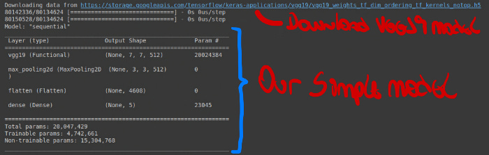
Now, we can fit the model. I use some callback to help our fitting. For example, save the best models during the fitting, early stopper, learning rate reduction and only 15 epochs are enough.
nome_modelo = 'modelo_VGG19_custom.h5'
checkpointer = ModelCheckpoint(nome_modelo, verbose=1, save_best_only=True) # Salvar os melhores modelos
early_stopper = EarlyStopping(patience = 5, monitor='val_loss')
learning_rate_reduction = ReduceLROnPlateau(
    monitor='val_accuracy',
    factor=0.3,
    min_lr=0.000001)
callbacks = [checkpointer, early_stopper, learning_rate_reduction]epochs = 15
batch_size = 64history = model.fit(
    x_train,y_train,
    batch_size = batch_size ,
    epochs = epochs ,
    validation_data = (x_test, y_test),
    callbacks = [callbacks])
Ok! After fitting, we need to evaluate the model.
epochs = [i for i in range(15)]
fig , ax = plt.subplots(1,2)
train_acc = history.history['accuracy']
train_loss = history.history['loss']
val_acc = history.history['val_accuracy']
val_loss = history.history['val_loss']
fig.set_size_inches(20,10)ax[0].plot(epochs , train_acc , 'go-' , label = 'Training Accuracy')
ax[0].plot(epochs , val_acc , 'ro-' , label = 'Testing Accuracy')
ax[0].set_title('Training & Testing Accuracy')
ax[0].legend()
ax[0].set_xlabel("Epochs")
ax[0].set_ylabel("Accuracy")ax[1].plot(epochs , train_loss , 'g-o' , label = 'Training Loss')
ax[1].plot(epochs , val_loss , 'r-o' , label = 'Testing Loss')
ax[1].set_title('Training & Testing Loss')
ax[1].legend()
ax[1].set_xlabel("Epochs")
ax[1].set_ylabel("Loss")
plt.show()
Nicceee, our model apparently is Ok! No overfitting. But, how generalist is it? We need to check the classification report and coffusion matrix.

Note that in the classification there is a good generalization. Each class has a high f1-score and this is ratified in the confusion matrix. Nice!!
And … finally, how our VGG19 classifies new images — Do you remember the valid dataset? We’ll use it now.
valid_df.reset_index(inplace=True)for (i, classe), cat in zip(enumerate(valid_df['Path']), valid_df['Categorical']):
  img_test = cv2.imread(valid_df.iloc[i]['Path'], cv2.IMREAD_COLOR)
  resized_image_test= cv2.resize(img_test, (img_size, img_size))
  x = np.array(resized_image_test) / 255
  x = x.reshape(-1, img_size, img_size, 3)
  real_predictions = model.predict(x)
  plt.imshow(img_test)
  plt.axis('off')
  plt.title(f"Classe Real : {cat}\n Classe Predita: {np.argmax(real_predictions)} ")
  plt.tight_layout()
  plt.show()


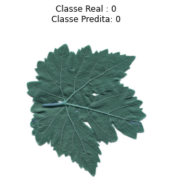
In general our model is a good classification. Sometimes it works and sometimes it goes wrong, but it is more often rigth than wrong, lol. In the next post I will show you how to deploy this model by using streamlit cloud. Byyee!
References:
https://neptune.ai/blog/transfer-learning-guide-examples-for-images-and-text-in-keras
https://iq.opengenus.org/vgg19-architecture/
https://www.sciencedirect.com/science/article/abs/pii/S0263224121013142?via%3Dihub
https://medium.com/mlearning-ai/mlearning-ai-submission-suggestions-b51e2b130bfb