
Resnet from scracth with Keras

In this post we’ll study about deep learning architecture Resnet and we’ll apply this archicteture in simple lemon quality dataset and classify some imagens. Let’s rock.
ResNet:
Create by Kaiming, Resnet won the ILSVRC 2015 challenge using a Residual Network, that delivered an astounding top-five error under 3.6%. The winning variant used an extremely deep CNN composed of 152 layers (other variantes had 34, 50 and 101 layers). It confirmed the general trend: models are getting deeper and deeper, with fewer and fewer parameters. The key to being able to train such a deep network is to use skip connections, also cales shortcut connections: the signal feeding into a layer is also added to the output of a layer located a bit higher up the stack. Let’s see why this is useful.
The aim when training a neural network is to make it model the target function h(x). If you add the input x to the network's output, the network will be forced to model f(x) = h(x) - x rather than h(x). This is called residual learning.
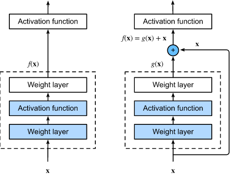
When initializing a traditional neural network, its weights are set close to zero, resulting in outputs close to zero. By adding a skip connection, the network outputs a duplicate of its inputs, effectively modeling the identity function. This can greatly accelerate training, particularly when the target function is close to the identity function, which is often the case.
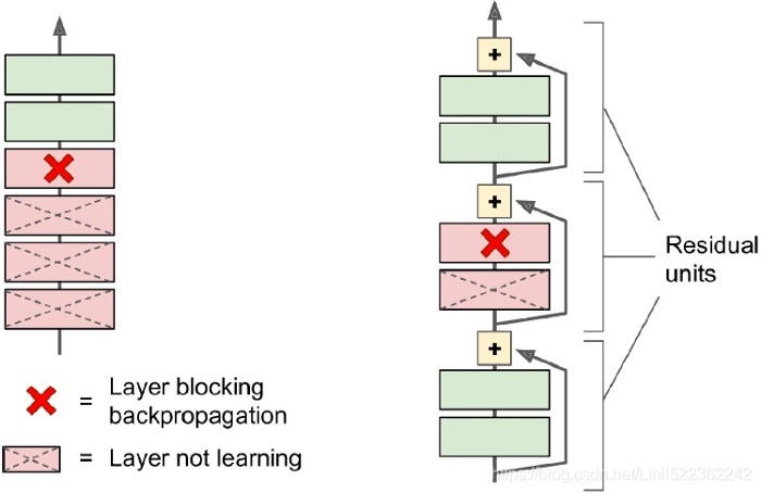
Additionally, adding multiple skip connections allows the network to make progress even if some layers have not begun learning yet. The skip connections facilitate the flow of signals throughout the network. A deep residual network can be thought of as a stack of residual units (RUs), each consisting of a small network with a skip connection.
The architecture of RenNet is simple. It begins and ends similarly to GoogleNet, but without a dropout layer, and in between is just a very deep stack of simple residual units. Each residual unit consists of two convolutional layers without a pooling layer, with batch normalization and ReLU activation, using 3x3 kernels while preserving spatial dimensions.
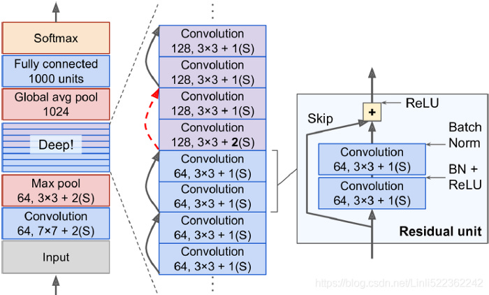
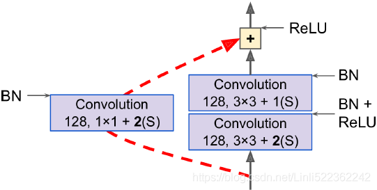
Note that the number of feature maps is doubled every few residual units, at the same time as their height and width are halved, using a convolutional layer with stride 2. When this happens, the inputs cannot be added directly to the outputs of the residual unit because they don’t have the same shape, for example, the problem affects the skip connection represented by the dashed arrow in the lat figure. To solve this problem, the inputs are passed through a 1x1 convolutional layer with stride 2 and the right number of output feature maps.
ResNet-34 is the ResNet with 34 layers (only counting the convolutional layers and the fully connected layer) containing 3 residual units that output 64 feature maps, 4 RUs with 128 maps, 6 RUs 256 maps, and 3 RUs with 512 maps. We’ll implement this architecture later.
ResNets deeper than that, such as ResNet-152, use slightly different resisual units. Instead of two 3x3 convolutional layers with, say 256 feature maps, they use three convolutional layers: first a 1x1 convolutional layer with just 64 feature maps (4 time less), wich acts as a bottleneck layer, then a 3x3 layer with 64 feature maps, and finally another 1x1 convolutional layer with 256 feature maps (4 time 64) that restores the original depth. ResNet-152 contains 3 such RUs that output 256 maps, then 8 RUs with 512 maps, a whopping 36 RUs with 1024 maps, and finally 3 RUs with 2048 maps.
One of the problems ResNets solve is the famous known vanishing gradient. This is because when the network is too deep, the gradients from where the loss function is calculated easily shrink to zero after several applications of the chain rule. This result on the weights never updating its values and therefore, no learning is being performed.
Dataset:
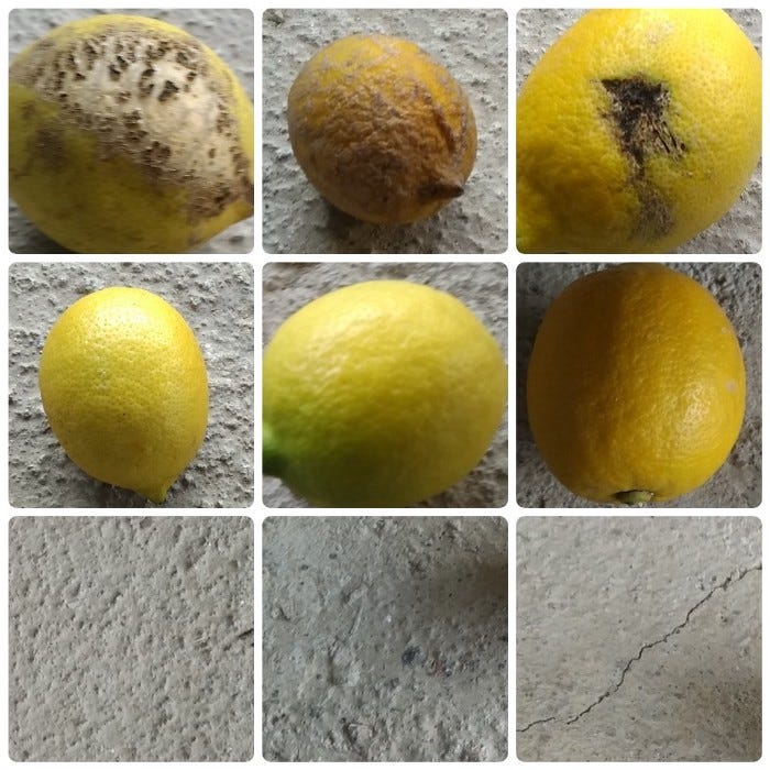
Our dataset is a kaggle dataset called Lemon dataset. This dataset has been prepared to investigate the possibilities to tackle the issue of fruit quality control. It contains 2.533 images (300 x 300 pixels). Lemon images are taken on a concrete surface. Dataset also includes empty images of this surface.
Dataset contains images of both bad and good quality lemons under slightly different lighting conditions (all under daylight) and sizes.
Code:
So, let’s go to our code. First thing to do is download correct libraries that we ‘ll use and download our dataset. Ah! Everything that we’ll do are make in google colab environment. If we go to the kaggle.com, you can download your json credentials, so do this and upload this file in your colab, because we’ll use this to download the lemon-quality-dataset. After, execute the code below.
import os# Lendo as crendenciais para download do dataset
os.environ['KAGGLE_CONFIG_DIR'] = "/content"!chmod 600 /content/kaggle.json# Download do dataset
!kaggle datasets download -d yusufemir/lemon-quality-dataset#Descompressao do dataset
!unzip /content/lemon-quality-dataset.zip -d /content/kaggle/
The next step is import the libriares that we’ll use and read our dataset
import numpy as np
import pandas as pd
from PIL import Image
import matplotlib.pyplot as plt
import cv2
import tensorflow as tf
from tensorflow import keras
from keras_preprocessing.image import ImageDataGenerator
import warnings
warnings.filterwarnings("ignore")
import os
for dirname, _, filenames in os.walk('/content/kaggle/lemon_dataset'):
    for filename in filenames:
        print(os.path.join(dirname, filename))
        pass
Now we’ll create a folder. That folder is where we’ll put the lemon with good quality class and the bad quality class, and prepare our image dataset.
%mkdir ./training/
%cp -R /content/kaggle/lemon_dataset/good_quality ./training/good_quality
%cp -R /content/kaggle/lemon_dataset/bad_quality ./training/bad_qualitybasePath = "/content/training"images = {}for dirname, dirlist, filenames in os.walk(basePath):
    lamon_class = dirname.split('/')[-1]
    if dirname != basePath and lamon_class in ['good_quality', 'bad_quality']:
        print(f"Number of {lamon_class} images: {len(filenames)}")
        filePaths = []
        for filename in filenames:
            filePaths.append(os.path.join(basePath, dirname, filename))
        images[lamon_class] = filePaths
We can plot some images of our dataset.
fig, ax = plt.subplots(2, 3, figsize=(18, 8))for i in range(6):
    img1 = cv2.imread(images[list(images.keys())[i//3]][i%3])
    img1 = cv2.cvtColor(img1, cv2.COLOR_BGR2RGB)
    ax[i//3][i%3].imshow(img1)
    ax[i//3][i%3].set_title(list(images.keys())[i//3])
    ax[i//3][i%3].axis('off')plt.show()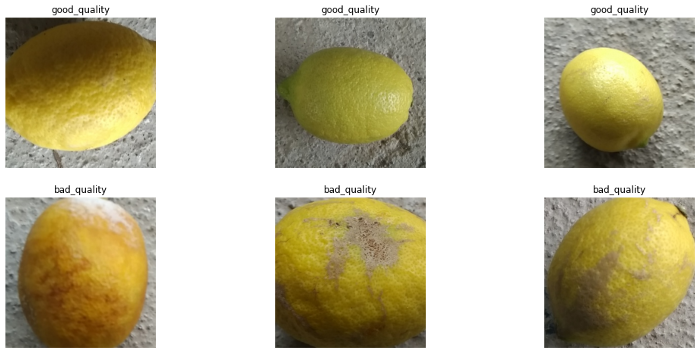
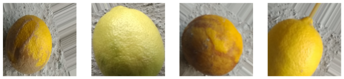
Now we’ll use Keras API to create data augmentation images. That’s necessary because we’ll make a really deep neural network. Let’s check the python script.
TRAINING_DIR = "./training"training_datagen = ImageDataGenerator(
    rescale = 1./255,
    rotation_range=40,
    width_shift_range=0.2,
    height_shift_range=0.2,
    shear_range=0.2,
    zoom_range=0.2,
    horizontal_flip=True,
    fill_mode='nearest',
    validation_split=0.2)
Notes that we’ll rotate the images, shift, flip and we’ll separete a validation part. The next figure show us some samples with this data augmentation.
Now we need separate our dataset in train and validation.
print('Traning Generator: ', end="")
train_generator = training_datagen.flow_from_directory(
    TRAINING_DIR,
    target_size=(224, 224),
    class_mode='binary',
    batch_size=1,
    subset='training'
)print('Validation Generator: ', end="")
validation_generator = training_datagen.flow_from_directory(
    TRAINING_DIR,
    target_size=(224, 224),
    batch_size=1,
    class_mode='binary',
    subset='validation')
Ok, next step is the part important this post. To create our ResNet Model. First we’ll make a class calls ResidualUnit. Most CNN architectures described so far are fairly straightfoward to implement (although generally you would load a pretrained network instead). To illustrate the process, let’s implement a ResNet-34 from scratch using Keras.
class ResidualUnit(keras.layers.Layer):
  def __init__(self, filters, strides=1, activation="relu", **kwargs):
    super().__init__(**kwargs)
    self.activation = keras.activations.get(activation)
    self.main_layers = [
        keras.layers.Conv2D(filters, 3, strides=strides, padding="same", use_bias=False),
        keras.layers.BatchNormalization(),
        self.activation,
        keras.layers.Conv2D(filters, 3, strides=1, padding="same", use_bias=False),
        keras.layers.BatchNormalization()
    ]
    self.skip_layers = []
    if strides > 1:
      self.skip_layers = [
          keras.layers.Conv2D(filters, 1, strides=strides, padding="same", use_bias=False),
          keras.layers.BatchNormalization()
      ]def get_config(self):
        config = super().get_config().copy()
        config.update({
            'activation': self.activation,
            'main_layers': self.main_layers,
            'skip_layers': self.skip_layers,
        })
        return configdef call(self, inputs):
    Z = inputs
    for layer in self.main_layers:
      Z = layer(Z)
      skip_Z = inputs
    for layer in self.skip_layers:
      skip_Z = layer(skip_Z)

    return self.activation(Z + skip_Z)
In the constructor, we create all the layers we will need: the main layers are the ones on the right side of the diagram, and the skip layers are the ones on the left (only needed if the stride is greater than 1). Then in the call() method, we make the inputs go through the main layers and the skip layers (if any), then we add both outputs and apply the activations function.
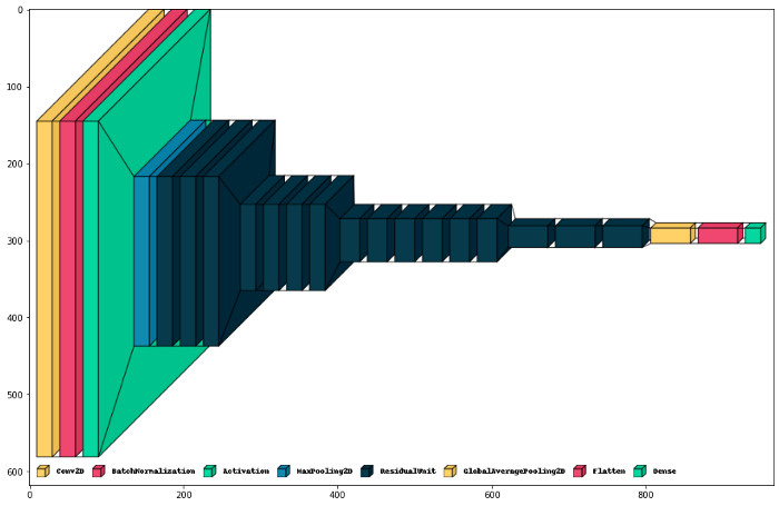
Next, we can build the ResNet-34 using a Sequential model, since it’s really just a long sequence of layers (we can trat each residual unit as a single layer now that we have the ResidualUnit class):
model = keras.models.Sequential()model.add(keras.layers.Conv2D(64, 7, strides=2, input_shape=[224, 224, 3]))
model.add(keras.layers.BatchNormalization())
model.add(keras.layers.Activation("relu"))
model.add(keras.layers.MaxPool2D(pool_size=3, strides=2, padding="same"))
prev_filters = 64
for filters in [64]*3 + [128]*4 + [256]*6 + [512]*3:
  strides = 1 if filters == prev_filters else 2
  model.add(ResidualUnit(filters, strides=strides))
  prev_filters = filters
model.add(keras.layers.GlobalAvgPool2D())
model.add(keras.layers.Flatten())
model.add(keras.layers.Dense(1, activation="sigmoid"))
model.summary()
The only slightly tricky part in this code is the loop that adds the ResidualUnit layers to the model: as explained earlier, the first 3 RUs have 64 filters, the the next 4 RUs have 128 filters, and so on. We the set the stride to 1 when the number of filters is the same as in the previous RU, or else we set it to 2. Then we add the ResidualUnit, and finally we update prev_filters. We can check the our ResNet’s architecture .
Now we can compile and train our model.
model.compile(
    loss='binary_crossentropy',
    optimizer='adam',
    metrics=['accuracy']
    )

BATCH_SIZE = 8history_custom = model.fit(
    train_generator,
    batch_size=BATCH_SIZE,
    epochs=20,
    validation_data=validation_generator,
    verbose=1
    )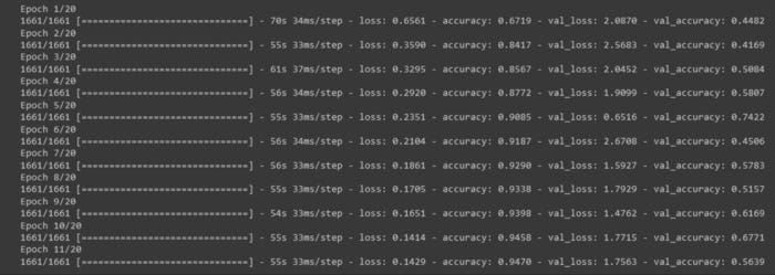
Now, we need to check our loss and accuracy curve.
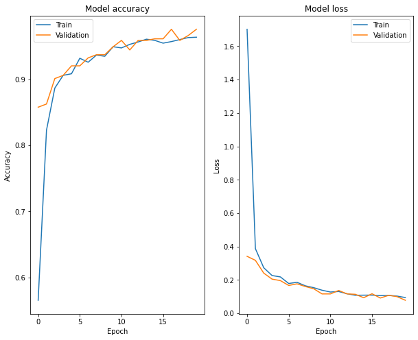
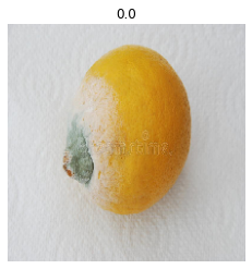
It’s ok! Our model prove itself well. But we need to do some inferece. To this I downloaded soma image lemon in the internet and make a prediction. We know that good quality is 1 and bad quality is 0.
!wget https://thumbs.dreamstime.com/b/lim%C3%A3o-podre-63225986.jpgfrom tensorflow.keras.preprocessing import imagetest_image = image.load_img('/content/limão-podre-63225986.jpg', target_size=(224, 224, 3))
test_image = image.img_to_array(test_image)
test_image = np.expand_dims(test_image, axis=0)
prediction = model.predict(test_image)train_generator.class_indices
prediction
Conclusion:
It is amazing that in fewer than 40 lines of code, we can build the model that won the ILSVRC 2015 challenge! This demonstrates both the elegance of the ResNet model and the expressiveness of the Keras API. Implementing th other CNN architectures is not much harder.
References:
[1]https://visio.ai/deep-learning/resnet-residual-neural-network/
[2]Hans-On: Machine Learning with Scikit-Learn, Keras and Tensorflow — 2nd Edition — Aurélien Géron
[3]Deep Resiual Learning for Image Recognition — article(https://arxiv.org/pdf/1512.03385.pdf)
[4]
https://keras.io/