Image Segmentation with watershed using Python
Imagine you need to segment some objects in an image, how to do that? In this post I will show you how to use a classic segmentation technique called watershed to do this.
What is watershed segmentation?
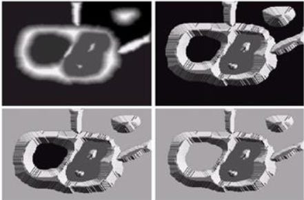
Watershed segmentantion is one of the most popular algorithm for image segmentation, normally used when we want to resolve one of the most difficult operations in image processing — separating similar objects in the image that are touching each other. For us to understand it easily, think of a grayscale image as a topographic surface, and in this image high-intensity pixel values represent peaks (white areas), whereas low-intensity values represent valleys — local minima (black areas).
So imagine now that we start filling the whole valley with water, and after a while the water coming up from different valleys will start to merge. To avoid this, we need to build barriers at the places where the water would merge, so the barriers are called basin lines and are used to determine the boundaries of the segment. When the water filling fills from the highest peak we stop the water filling. At the end of the process, only the watershed lines will be visible and this will be the final result of the segmentation. Thus, the purpose of the watershed is to identify watershed lines and segmented image.
In essence, we partition the image into two different sets:
catchment basins — dark areas; The group of connected pixels with the same local minimum.
watershed lines — Lines that divide one catchment area from another .
So, what’s the watershed algorithm pipeline?
1. Binary image
2. Calculate a distance transform
3. Find local maxima points
4. Label the marks
I Think it would be easier to show this pipeline together with Python’s code. First, let’s import the necessary libraries and do the image pre-processing.
| import cv2 | |
| import numpy as np | |
| from scipy import ndimage as ndi | |
| from skimage.feature import peak_local_max | |
| from skimage.segmentation import watershed | |
| import matplotlib.pyplot as plt | |
| img = cv2.imread('coins.jpg') | |
| gray = cv2.cvtColor(img, cv2.COLOR_BGR2RGB) | |
| filtro = cv2.pyrMeanShiftFiltering(img, 20, 40) | |
| gray = cv2.cvtColor(filtro, cv2.COLOR_BGR2GRAY) | |
| _, thresh = cv2.threshold(gray, 0, 255, cv2.THRESH_BINARY_INV | cv2.THRESH_OTSU) |
Our image test are coins and our goal is segment this coins.
Let’s fill all hole that can be small (area is less than 1000 pixels).
| contornos, _ = cv2.findContours(thresh, cv2.RETR_TREE, cv2.CHAIN_APPROX_SIMPLE) | |
| buracos = [] | |
| for con in contornos: | |
| area = cv2.contourArea(con) | |
| if area < 1000: | |
| buracos.append(con) | |
| cv2.drawContours(thresh, buracos, -1, 255, -1) |
We now need to try to separate the touching objects and try to create a border betweeb them. One idea is to create a border as far as possible from the centers of the overlapping objects. Then, we’ll use a thecnique called distance transform. It is an operator that generally takes binary images as inputs and pixel intensities of the points inside the foreground regions are replaced by their distance to the nearest pixel with zero intensity (background pixel). We can use the fucntion distance_transform_edt() from scipy library. This fucntion calculate the exact Euclidean distance transform.
| dist = ndi.distance_transform_edt(thresh) | |
| dist_visual = dist.copy() |
If we plot the original image, binary image and the distance transform we’ll see this image below.
Notes that in the distance transform we can see white pixels closets to the center, these pixels are larger distance transform value.
Now we need to find the coordinates of the peaks (local maxima) of the white areas in the image. For that, we will use the function peak_local_max()from the Scikit-image library. We will apply this function to our distance_transform image and the output will give us the markers which will be used in the watershed function.
| local_max = peak_local_max(dist, indices=False, min_distance=20, labels=thresh) |
Let’s continue with our code. The next step is to label markers for the watershed function. For that, we will use the function ndi.label()from the SciPy library. This function consists of one parameter input which is an array-like object to be labeled. Any non-zero values in this parameter are considered as features and zero values are considered to be the background. In our code, we will use the coordinates of the calculated local maximum. Then, the function ndi.label()will randomly label all local maximums with different positive values starting from 1. So, in case we have 10 objects in the image each of them will be labeled with a value from 1 to 10.
| markers = ndi.label(local_max, structure=np.ones((3, 3)))[0] |
The final step is to apply the skimage.segmentation.watershed()function from the Scikit-image library. As parameters, we need to pass our inverted distance transform image and the markers that we calculated in the previous line of code. Since the watershed algorithm assumes our markers represent local minima we need to invert our distance transform image. In that way, light pixels will represent high elevations, while dark pixels will represent the low elevations for the watershed transform.
| labels = watershed(-dist, markers, mask=thresh) |
And finally, we will plot our original image, binary Image, distance transform image, and the watershed image.
| titulos = ['Original image', 'Binary Image', 'Distance Transform', 'Watershed'] | |
| imagens = [img, thresh, dist_visual, labels]fig = plt.gcf() | |
| fig.set_size_inches(16, 12) | |
| for i in range(4): | |
| plt.subplot(2,2,i+1) | |
| if (i == 3): | |
| cmap = "jet" | |
| else: | |
| cmap = "gray" | |
| plt.imshow(imagens[i], cmap) | |
| plt.title(titulos[i]) | |
| plt.xticks([]),plt.yticks([]) | |
| plt.show() |
References:
https://datahacker.rs/007-opencv-projects-image-segmentation-with-watershed-algorithm/
https://docs.opencv.org/4.x/d3/db4/tutorial_py_watershed.html


